Using symptom analysis, this study employs a Random Forest approach to predict severity levels in patients, aiming to enhance healthcare decision-making.
Author
Brian Cervantes Alvarez
Published
June 26, 2023
Modified
August 11, 2025
Yapper Labs | AI Summary
Model: ChatGPT 4.5
I conducted symptom-based severity prediction using a Random Forest model, performing exploratory analysis, strategic feature engineering, and comprehensive evaluations. I successfully classified patient severity into Mild, Moderate, and Severe categories, achieving strong model performance metrics (ROC AUC = 0.95, Recall = 90%, Precision = 91.3%, Kappa = 0.85). These results enable personalized healthcare strategies by providing clear classification rules based on symptoms.
Abstract
This paper presents a machine learning study that aims to predict severity levels in patients by utilizing a random forest approach based on symptom analysis. The objective of the study was to develop accurate rules for classifying patients into three severity levels: Mild, Moderate, and Severe. The dataset consisted of patient symptoms, which were used in conjunction with a random forest model for the classification task. The results indicated that patients with 1 to 3 symptoms, including depression, were classified as Mild, while those with at least 3 symptoms, including depression and cramps, were classified as Moderate. Patients with 4 symptoms, including cramps and spasms, were classified as Severe. The study conducted comprehensive evaluations using metrics such as the confusion matrix, ROC AUC, precision vs recall, and kappa to assess the performance of the random forest model. The results highlighted the promising performance of the model in accurately predicting severity levels among patients. The findings from this study provide robust evidence that can contribute to personalized healthcare and effective treatment planning.
Introduction
In the field of rare diseases, physicians often observe variations in the severity levels of patients; however, there is a lack of established guidelines to map individual patients directly to specific severity levels. Our client, who is developing a product for this rare disease, aims to target patients with moderate to severe conditions. To address this challenge, the client possesses a comprehensive database containing clinically relevant information about the disease, including symptom flags and a symptom count variable. Additionally, each patient in the database has been rated by a physician as mild, moderate, or severe. The client has approached [REDACTED] with the objective of extracting the mental heuristics employed by physicians when assigning severity labels to patients. The task at hand involves deriving simple rules (1-3 per severity level) from the database that can effectively classify patients. For instance, a set of rules might involve identifying patients as severe if they exhibit fatigue or have exactly two symptoms. By extracting these rules, our aim is to provide the client with a clearer understanding of the factors influencing severity levels in order to enhance their product development and enable more personalized patient care.
Methodology
# Import the required librariesimport pandas as pd # Library for data manipulation and analysisimport numpy as np # Library for numerical computationsimport matplotlib.pyplot as plt # Library for data visualizationimport seaborn as sns# Import Machine Learning librariesfrom sklearn import tree # Library for decision tree modelsfrom sklearn.ensemble import RandomForestClassifier # Library for random forest modelsfrom sklearn.model_selection import ( cross_val_score, # Library for cross-validation train_test_split, GridSearchCV) from sklearn.preprocessing import LabelEncoder # Library for label encodingfrom sklearn.metrics import ( # Library for model evaluation metrics confusion_matrix, # Confusion matrix roc_auc_score, # ROC AUC score roc_curve, # ROC Curve plot recall_score, # Recall score precision_score, # Precision score precision_recall_curve, # Recall vs. Precision Curve cohen_kappa_score # Cohen's kappa score)# Load the datasetds = pd.read_csv("../../../assets/datasets/severityLevels.csv") ds.head(10) # Display the first 10 rows of the dataset
Patient
Final Category
Fatigue
Weakness
Depression
Anxiety
Dry Skin
Spasms
Tingling
Headaches
Cramps
Number of Symptoms
0
1
Mild
0
0
1
0
0
0
0
0
0
1
1
2
Mild
0
0
0
0
0
0
1
1
0
2
2
3
Mild
1
0
0
0
1
0
1
1
0
4
3
4
Mild
0
0
0
0
0
0
0
0
0
0
4
5
Mild
0
0
0
0
0
0
1
0
0
1
5
6
Mild
1
0
0
0
0
0
0
0
0
1
6
7
Mild
0
0
0
0
0
0
0
0
0
0
7
8
Mild
0
0
1
0
0
0
0
1
0
2
8
9
Mild
1
0
0
0
0
0
1
0
0
2
9
10
Mild
0
0
0
0
1
0
0
0
0
1
Exploratory Data Analysis
# Display basic statistics of the datasetds.describe()
Patient
Fatigue
Weakness
Depression
Anxiety
Dry Skin
Spasms
Tingling
Headaches
Cramps
Number of Symptoms
count
300.000000
300.000000
300.000000
300.000000
300.000000
300.000000
300.000000
300.000000
300.000000
300.000000
300.000000
mean
150.500000
0.466667
0.396667
0.356667
0.363333
0.366667
0.200000
0.323333
0.333333
0.213333
3.020000
std
86.746758
0.499721
0.490023
0.479816
0.481763
0.482700
0.400668
0.468530
0.472192
0.410346
1.703704
min
1.000000
0.000000
0.000000
0.000000
0.000000
0.000000
0.000000
0.000000
0.000000
0.000000
0.000000
25%
75.750000
0.000000
0.000000
0.000000
0.000000
0.000000
0.000000
0.000000
0.000000
0.000000
2.000000
50%
150.500000
0.000000
0.000000
0.000000
0.000000
0.000000
0.000000
0.000000
0.000000
0.000000
3.000000
75%
225.250000
1.000000
1.000000
1.000000
1.000000
1.000000
0.000000
1.000000
1.000000
0.000000
4.000000
max
300.000000
1.000000
1.000000
1.000000
1.000000
1.000000
1.000000
1.000000
1.000000
1.000000
8.000000
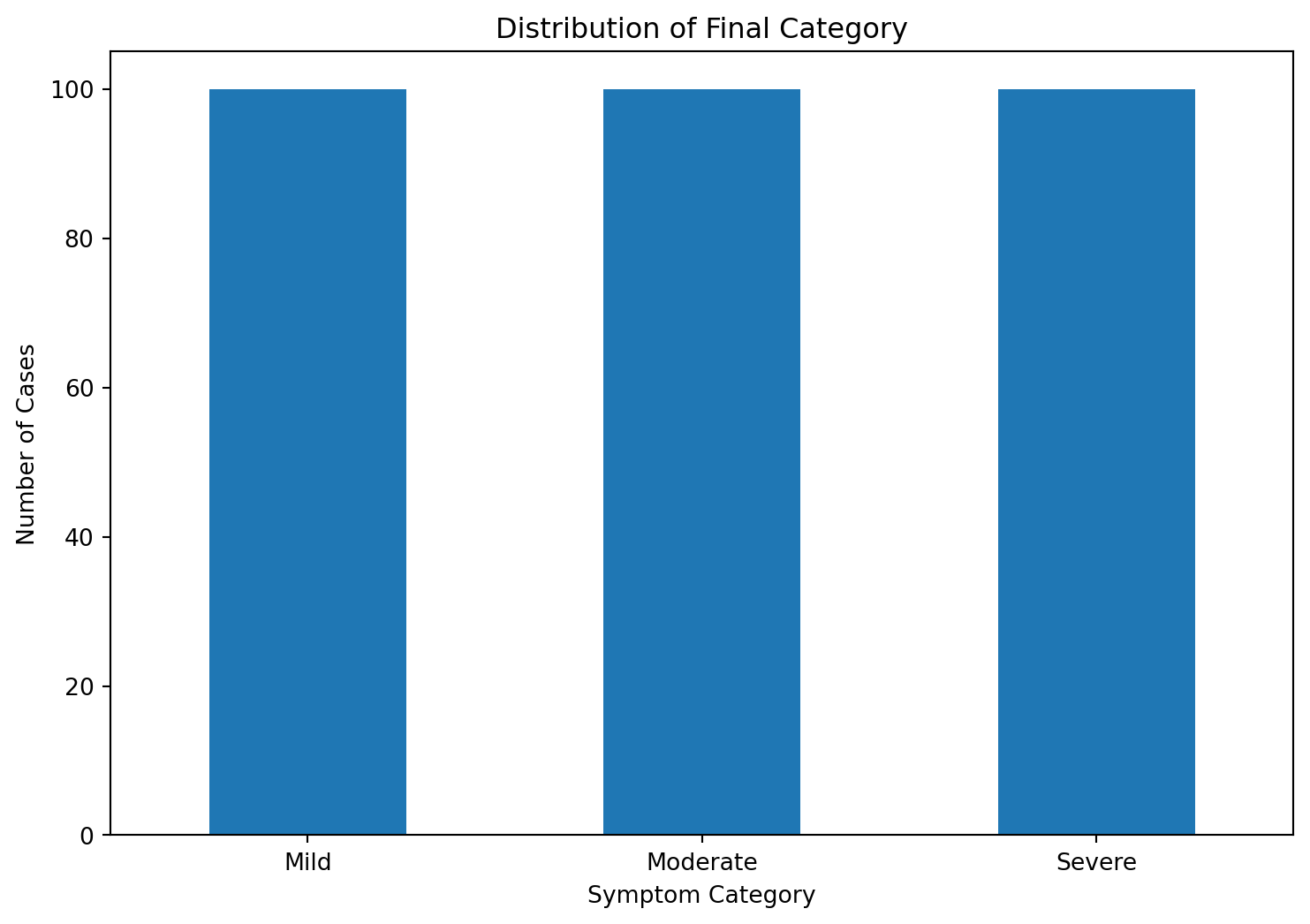
# Visualize the distribution of the target variable 'Final Category'plt.figure(figsize=(9, 6))ds['Final Category'].value_counts().plot(kind='bar')plt.xlabel('Symptom Category')plt.ylabel('Number of Cases')plt.title('Distribution of Final Category')plt.xticks(rotation=0) # Set rotation to 0 degrees for horizontal x-axis labelsplt.show()plt.clf()plt.close()plt.show()
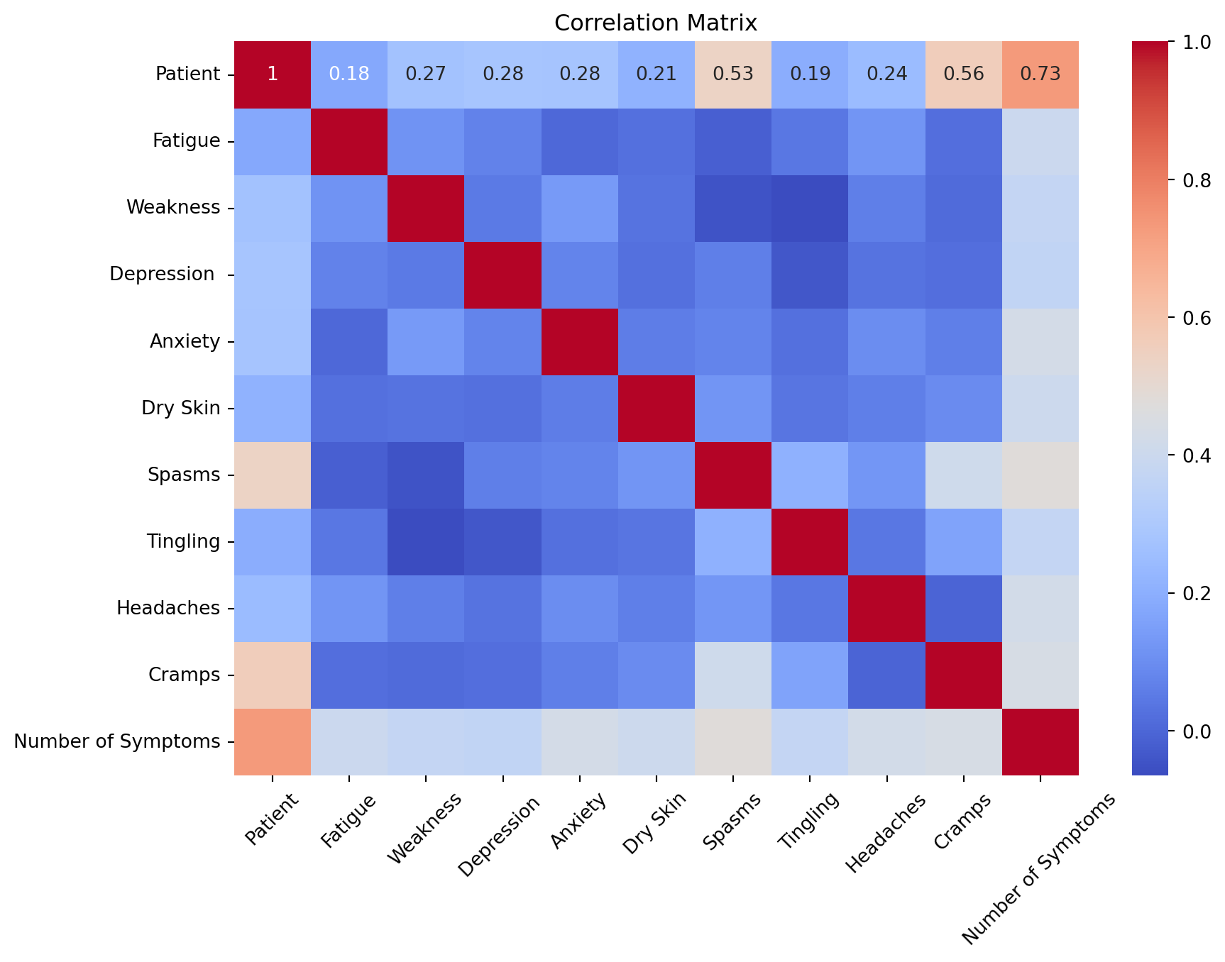
# Calculate the correlation matrix# Select only numeric columnsnumeric_ds = ds.select_dtypes(include='number')# Calculate the correlation matrixcorr_matrix = numeric_ds.corr()# Visualize the correlation matrixplt.figure(figsize=(10, 7))sns.heatmap(corr_matrix, annot=True, cmap='coolwarm')plt.title('Correlation Matrix')plt.xticks(rotation=45)plt.show()
Feature Engineering
The code performs some data preprocessing and feature selection to prepare the data for a Random Forest model. Let’s go through each step:
Drop the ID column: The code removes a column named “Patient” from the dataset. This column likely contains unique identifiers for each patient, and since it’s not relevant for our analysis, we can safely remove it.
Create dummy columns for “Number of Symptoms”: The code converts a column called “Number of Symptoms” into multiple binary columns, known as dummy variables. Each dummy variable represents a unique value in the original column. This transformation helps us to use categorical data in our machine learning model.
Concatenate the dummy columns with the original dataframe: The code combines the newly created dummy columns with the original dataset. This ensures that we retain all the existing information while incorporating the transformed categorical data.
Drop the original “Number of Symptoms” column: Since we have created the dummy columns, we no longer need the original “Number of Symptoms” column. Therefore, the code removes this column from the dataset.
Separate the features (X) and the target variable (y): The code splits the dataset into two parts. The features, represented by the variable X, contain all the columns except the “Final Category” column, which is the target variable we want to predict. The target variable, represented by the variable y, contains only the “Final Category” column. This is the severity cases of ‘Mild’, ‘Moderate’ and ‘Severe’
Perform feature selection using Random Forest: The code utilizes a machine learning algorithm called Random Forest to identify the most important features for each category in the target variable. It trains a separate Random Forest model for each category and determines the top three features that contribute the most to predicting that category.
Store the top features for each category: The code stores the top three features for each category in a dictionary called “top_features.” Each category is represented by a label, and the corresponding top features are stored as a list.
Print the top 3 features for each label: The code then prints the top three features for each category in the target variable. This information helps us understand which features are most influential in determining the predicted category.
Overall, this code prepares the data by transforming categorical data into a suitable format and identifies the top features that contribute to predicting different categories. This sets the stage for further analysis and building the final machine learning model based on these selected features.
# Drop the ID columnds.drop('Patient', axis=1, inplace=True)# Create dummy columns from the "Number of Symptoms" columndummy_cols = pd.get_dummies(ds['Number of Symptoms'], prefix='Symptom')# Concatenate the dummy columns with the original dataframeds = pd.concat([ds, dummy_cols], axis=1)# Drop the original "Number of Symptoms" columnds.drop('Number of Symptoms', axis=1, inplace=True)ds.head(10)
Final Category
Fatigue
Weakness
Depression
Anxiety
Dry Skin
Spasms
Tingling
Headaches
Cramps
Symptom_0
Symptom_1
Symptom_2
Symptom_3
Symptom_4
Symptom_5
Symptom_6
Symptom_7
Symptom_8
0
Mild
0
0
1
0
0
0
0
0
0
0
1
0
0
0
0
0
0
0
1
Mild
0
0
0
0
0
0
1
1
0
0
0
1
0
0
0
0
0
0
2
Mild
1
0
0
0
1
0
1
1
0
0
0
0
0
1
0
0
0
0
3
Mild
0
0
0
0
0
0
0
0
0
1
0
0
0
0
0
0
0
0
4
Mild
0
0
0
0
0
0
1
0
0
0
1
0
0
0
0
0
0
0
5
Mild
1
0
0
0
0
0
0
0
0
0
1
0
0
0
0
0
0
0
6
Mild
0
0
0
0
0
0
0
0
0
1
0
0
0
0
0
0
0
0
7
Mild
0
0
1
0
0
0
0
1
0
0
0
1
0
0
0
0
0
0
8
Mild
1
0
0
0
0
0
1
0
0
0
0
1
0
0
0
0
0
0
9
Mild
0
0
0
0
1
0
0
0
0
0
1
0
0
0
0
0
0
0
# Separate the features (X) and the target variable (y)X = ds.drop('Final Category', axis=1)y = ds['Final Category']# Split the data into training and testing setsX_train, X_test, y_train, y_test = train_test_split(X, y, test_size=0.2, random_state=42)# Initialize a dictionary to store top features per labeltop_features = {}# Perform feature selection for each labelfor label in y_train.unique():# Encode the target variable for the current label y_label_train = (y_train == label).astype(int) y_label_test = (y_test == label).astype(int)# Create a Random Forest model rf_model = RandomForestClassifier(random_state=60)# Train the model rf_model.fit(X_train, y_label_train)# Get feature importances feature_importances = rf_model.feature_importances_# Sort features by importance in descending order sorted_features =sorted(zip(X_train.columns, feature_importances), key=lambda x: x[1], reverse=True)# Get the top 3 features for the current label selected_features = [feature for feature, _ in sorted_features[:3]]# Store the top features for the current label top_features[label] = selected_features# Print the top 3 features for each labelfor label, features in top_features.items():print(f"Top 3 features for {label}:")print(features)print()
Top 3 features for Severe:
['Cramps', 'Spasms', 'Symptom_4']

Top 3 features for Mild:
['Depression ', 'Symptom_1', 'Symptom_3']

Top 3 features for Moderate:
['Symptom_3', 'Depression ', 'Cramps']
Features Explained
The feature selection process aims to identify the most important factors (features) that contribute to determining the severity of a patient’s condition. In this case, the severity levels are categorized as “Mild,” “Moderate,” and “Severe.” The top three features that were found to be most indicative for each severity level are as follows:
For patients rated as “Mild”:
Has 1 symptom:
This feature indicates the presence of a specific symptom (let’s say, symptom X) that is associated with a mild severity rating. If a patient has symptom X, it suggests a higher likelihood of being classified as “Mild.”
Depression:
This feature refers to the presence or absence of depression symptoms in the patient. The presence of depression symptoms is considered important in determining a mild severity rating.
Has 3 symptoms:
This feature represents the presence of 3 symptoms (let’s call them symptoms A,B,C) that are associated with a mild severity rating. If a patient has symptoms A,B,C, it suggests a higher likelihood of being classified as “Mild.”
Given this information, it can be recommended that a threshold is established. It can be inferred that if a patient has 1-3 symptoms and/or has depression, they can be classified as “Mild.” This is addressed with the model later in the study.
For patients rated as “Moderate”:
Has 3 symptoms:
This feature represents the presence of 3 symptoms (let’s call them symptoms A,B,C again) that are associated with a moderate severity rating. If a patient has symptoms A,B,C, it suggests a higher likelihood of being classified as “Moderate.”
Depression:
The presence or absence of depression symptoms also plays a role in determining a moderate severity rating.
Cramps:
This feature represents the presence or absence of cramps in the patient. The presence of cramps is considered important in predicting a moderate severity rating.
Given this information, another threshold can be established. It can be inferred that if a patient has at least 3 symptoms and/or has depression and/or cramps, they can be classified as “Moderate.” This is addressed with the model later in the study.
For patients rated as “Severe”:
Cramps:
This feature indicates the presence or absence of cramps, which is associated with a severe severity rating. If a patient has cramps, it suggests a higher likelihood of being classified as “Severe.”
Spasms:
This feature refers to the presence or absence of muscle spasms in the patient. The presence of spasms is considered important in predicting a severe severity rating.
Has 4 symptoms:
This feature represents the presence of symptoms (let’s call it symptoms A,B,C,D) that are associated with a severe severity rating. If a patient has symptoms , it suggests a higher likelihood of being classified as “Severe.”
Given this information, a last threshold can be established. It can be inferred that if a patient has at least 4 symptoms and/or has cramps and/or spasms, they can be classified as “Severe.” This is addressed with the model later in the study.
In summary, the top features identified for each severity level provide insights into the specific symptoms and factors that contribute to determining the severity of a patient’s condition. By considering the presence or absence of these features, the model can make predictions about the severity rating of a patient’s condition, helping healthcare professionals assess the level of severity and provide appropriate care and treatment.
Random Forest Model
The code performs machine learning tasks using a Random Forest model with the selected features from the earlier model. Let’s go through each step:
Separate the features (X) and the target variable (y) using only the top features: The code selects specific features from the dataset based on their importance in predicting the target variable. These features are obtained from the “top_features” dictionary, which contains the top three features for each category (Mild, Moderate, and Severe) in the target variable.
Encode the target variable using label encoding: The target variable “Final Category” is a categorical variable. To use it in the machine learning model, we need to convert it into numeric form. The code uses label encoding, which assigns a unique numeric value to each category in the target variable.
Create a random forest model using the top features: The code initializes a Random Forest model with a specific random state. Random Forest is an ensemble learning algorithm that combines multiple decision trees to make predictions.
Perform 10-fold cross-validation: The code evaluates the performance of the Random Forest model using a technique called cross-validation. Cross-validation helps estimate how well the model will generalize to new, unseen data. In this case, 10-fold cross-validation is performed, which means the dataset is divided into 10 equal parts (folds). The model is trained and tested 10 times, with each fold serving as the test set once.
Print the cross-validation scores: The code prints the cross-validation scores obtained from each fold. These scores indicate how well the model performed on each fold. Additionally, the mean cross-validation score is calculated, which provides an overall measure of the model’s performance.
Train the model: The code trains the Random Forest model using all the available data, as specified by the features (X) and target variable (y).
Make predictions on the training set: The code uses the trained model to make predictions on the same dataset that was used for training. This helps evaluate how well the model can predict the target variable for the given features.
Print the confusion matrix: The code prints a confusion matrix, which is a table that shows the number of correct and incorrect predictions made by the model. It provides insights into the model’s performance for each category in the target variable.
Calculate and print other evaluation metrics: The code calculates additional evaluation metrics such as ROC AUC score, recall, precision, and Kappa metric. These metrics help assess the model’s performance in terms of classification accuracy, sensitivity, precision, and agreement beyond chance.
Overall, this code builds a Random Forest model using selected features, evaluates its performance through cross-validation, and provides insights into the model’s predictive capabilities using various evaluation metrics. The goal is to understand how well the model can predict the categories in the target variable based on the selected features.
# Separate the features (X) and the target variable (y) using only the top featuresX = ds[top_features['Mild'] + top_features['Moderate'] + top_features['Severe']]y = ds['Final Category']# Encode the target variable using label encodinglabel_encoder = LabelEncoder()y = label_encoder.fit_transform(y)# Create a random forest modelrf_model = RandomForestClassifier(random_state=60)# Define the parameter grid for hyperparameter optimizationparam_grid = {'max_depth': [None],'min_samples_leaf': [4],'min_samples_split': [2],'n_estimators': [100]}# Perform hyperparameter optimization using grid search and 10-fold cross-validationgrid_search = GridSearchCV(rf_model, param_grid, cv=10)grid_search.fit(X, y)# Get the best random forest model with optimized hyperparametersrf_model = grid_search.best_estimator_# Perform 10-fold cross-validation with the optimized modelcv_scores = cross_val_score(rf_model, X, y, cv=10)# Print the cross-validation scoresprint("Cross-Validation Scores:", cv_scores)print("Mean CV Score:", cv_scores.mean())print()
# Split the data into training and testing setsX_train, X_test, y_train, y_test = train_test_split(X, y, test_size=0.2, random_state=87)# Train the modelrf_model.fit(X_train, y_train)# Make predictions on the test sety_pred = rf_model.predict(X_test)# Print confusion matrixprint("Confusion Matrix:")print(confusion_matrix(y_test, y_pred))print()# Calculate and print ROC AUC scoreroc_auc = roc_auc_score(y_test, rf_model.predict_proba(X_test), multi_class='ovr')print("ROC AUC:", roc_auc)print()# Calculate and print recall scorerecall = recall_score(y_test, y_pred, average='weighted')print("Recall:", recall)print()# Calculate and print precision scoreprecision = precision_score(y_test, y_pred, average='weighted')print("Precision:", precision)print()# Calculate and print Kappa metrickappa = cohen_kappa_score(y_test, y_pred)print("Kappa:", kappa)print()
Let’s break down the provided metrics based on the given confusion matrix:
Confusion Matrix
The confusion matrix is a table that helps us understand the performance of a classification model. It shows the predicted labels versus the actual labels for each class. In this case, the confusion matrix has three rows and three columns, representing the three severity rating categories. In this case, since I set the test set to be 20% of the sample of 300, there is 60 total patients that were randomly tested.
First, the number 18 in the first row and column indicates that the model correctly predicted 18 patients as “mild” which coincides with the actual “mild” severity label. Next, the number 4 in the first row and second column indicates that the model incorrectly predicted 4 patients as “moderate” when their actual severity rating was “mild.” Lastly, the number 0 in the first row and third column indicates that the model correctly predicted 0 patients as being “severe”, meaning that those patients were labeled correctly as “mild”.
Similarly, the other numbers in the confusion matrix represent the model’s predictions for the other severity rating categories. Given that this was a dataset with only 300 patients, it is very intriguing that it can label each patient with high accuarcy.
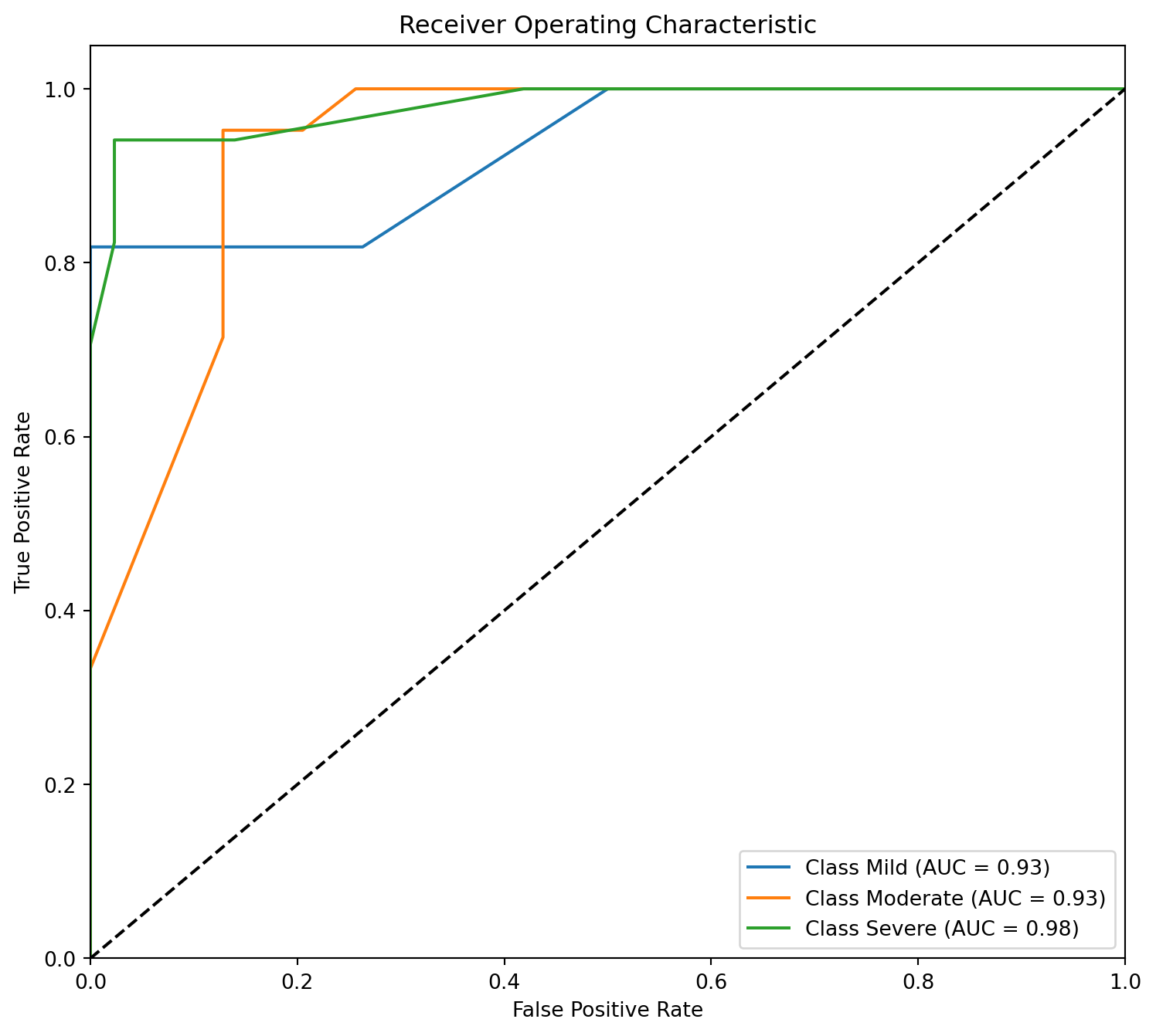
ROC Curve
Now, the ROC AUC (Receiver Operating Characteristic Area Under the Curve) is a measure of the model’s ability to distinguish between different severity ratings. It represents the overall performance of the model across all severity levels. The value of 0.948 indicates a high level of performance, close to 1, suggesting that the model has good predictive capability for distinguishing between severity ratings.
# Calculate predicted probabilities for each classy_pred_proba = rf_model.predict_proba(X_test)# Compute the ROC curve for each classfpr =dict()tpr =dict()roc_auc =dict()for class_index inrange(len(label_encoder.classes_)): fpr[class_index], tpr[class_index], _ = roc_curve( (y_test == class_index).astype(int), y_pred_proba[:, class_index] ) roc_auc[class_index] = roc_auc_score( (y_test == class_index).astype(int), y_pred_proba[:, class_index] )# Plot the ROC curve for each classplt.figure(figsize=(9, 8))for class_index inrange(len(label_encoder.classes_)): plt.plot( fpr[class_index], tpr[class_index], label=f"Class {label_encoder.classes_[class_index]} (AUC = {roc_auc[class_index]:.2f})", )# Plot random guessing lineplt.plot([0, 1], [0, 1], "k--")# Set plot propertiesplt.xlim([0.0, 1.0])plt.ylim([0.0, 1.05])plt.xlabel("False Positive Rate")plt.ylabel("True Positive Rate")plt.title("Receiver Operating Characteristic")plt.legend(loc="lower right")# Show the plotplt.show()plt.clf()plt.close()plt.show()
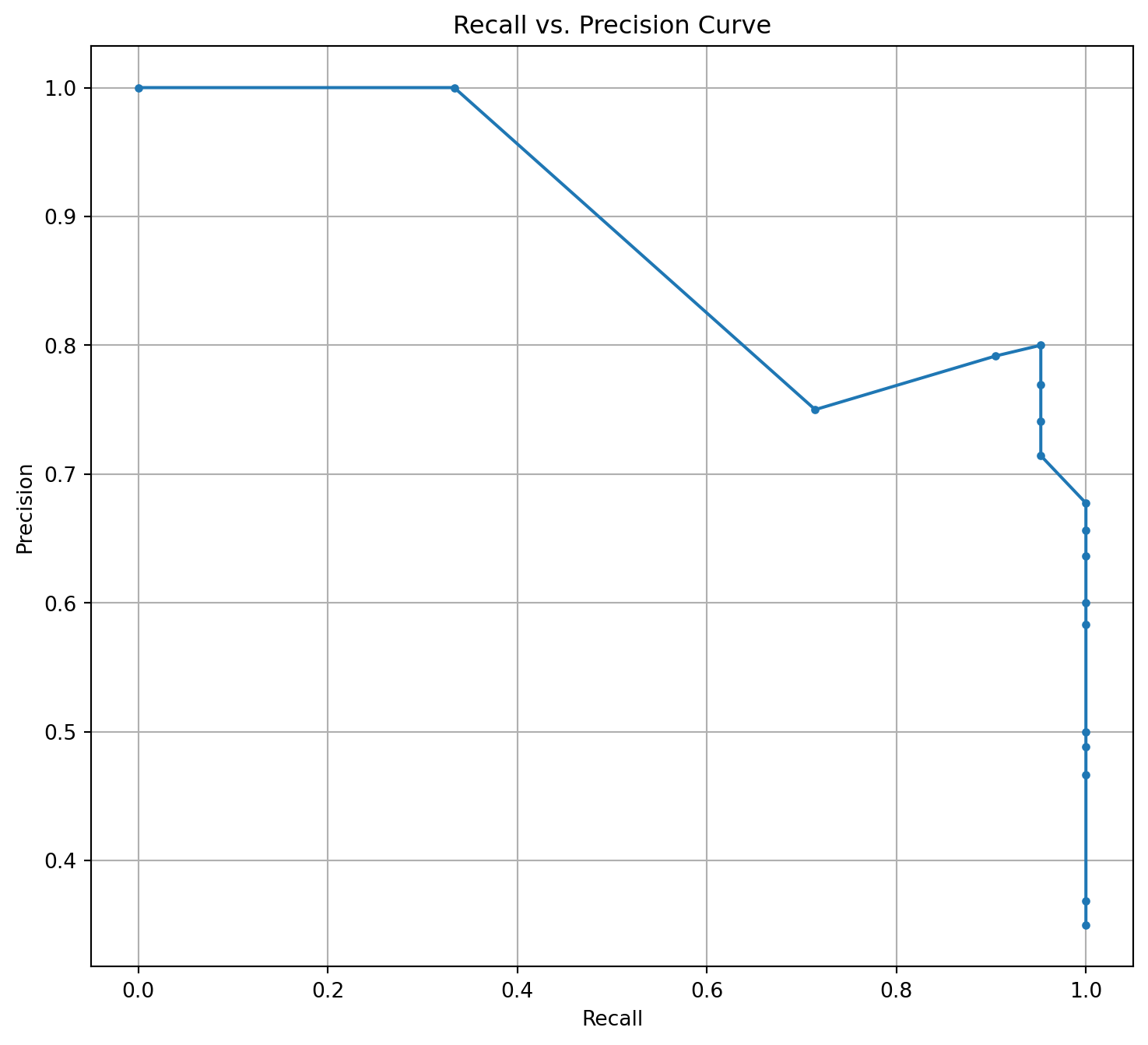
Recall vs. Precision Curve
Recall, also known as sensitivity or true positive rate, measures the proportion of actual positive instances (patients with a particular severity rating) that the model correctly identified. A recall value of 0.9 means that the model identified nearly 90.0% of the patients with their correct severity rating.
Precision measures the proportion of instances that the model predicted correctly as positive (patients with a particular severity rating) out of all instances it predicted as positive. A precision value of 0.913 indicates that out of all the patients the model identified as having a specific severity rating, 91.3% of them were correct.
# Calculate precision and recall values for each classprecision, recall, thresholds = precision_recall_curve(y_test, rf_model.predict_proba(X_test)[:, 1], pos_label=1)# Plot the recall vs. precision curveplt.figure(figsize=(9, 8))plt.plot(recall, precision, marker='.')plt.xlabel('Recall')plt.ylabel('Precision')plt.title('Recall vs. Precision Curve')plt.grid(True)plt.show()plt.clf()plt.close()plt.show()
Kappa
The Kappa statistic is a measure of agreement between the model’s predictions and the actual severity ratings, taking into account the possibility of agreement occurring by chance. A Kappa value of 0.849 indicates a substantial level of agreement between the model’s predictions and the actual severity ratings, suggesting a reliable performance of the model.
Overall, these metrics indicate that the model has performed well in predicting the severity ratings of the patients, with high accuracy, good distinction between severity levels, and substantial agreement with the actual severity ratings provided by physicians.
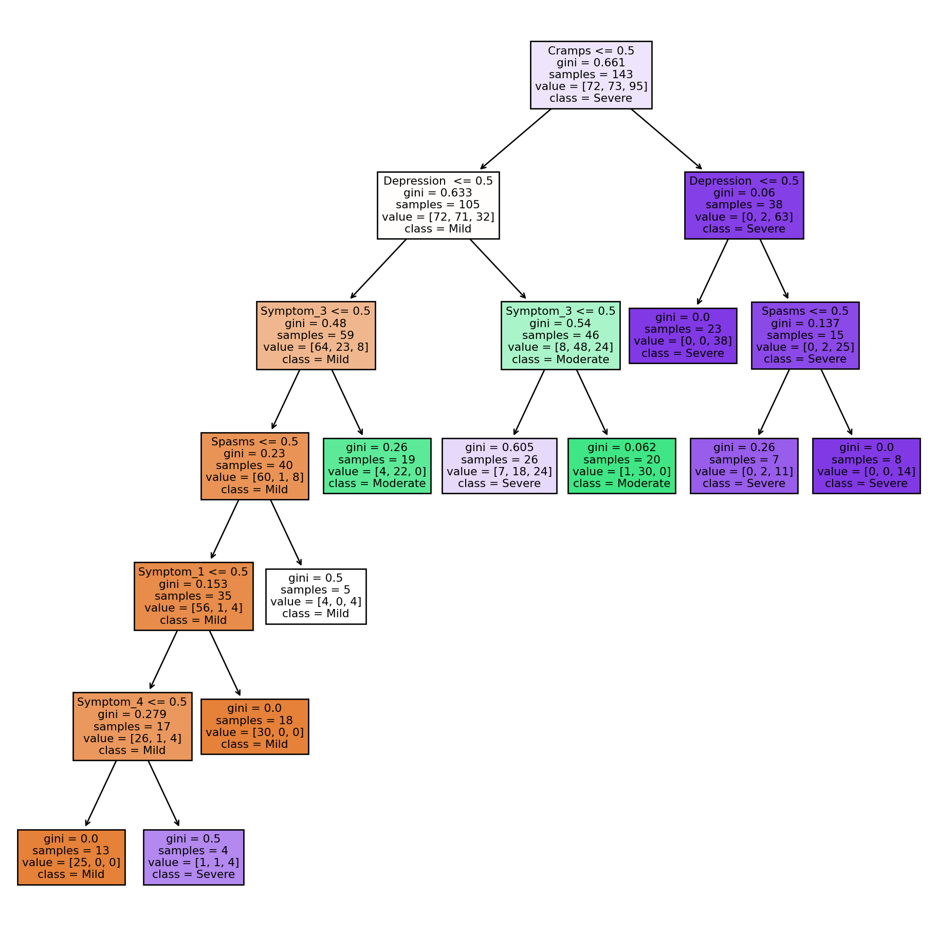
Visualizing Random Forest’s Best Decision Tree
# Perform 10-fold cross-validationcv_scores = cross_val_score(rf_model, X, y, cv=10)# Find the index of the best decision treebest_tree_index = np.argmax(cv_scores)# Get the best decision tree from the random forestbest_tree = rf_model.estimators_[best_tree_index]# Visualize the best decision tree using matplotlibplt.figure(figsize=(12, 12))tree.plot_tree(best_tree, feature_names=X.columns, class_names=label_encoder.classes_, filled=True)plt.show()
Results
If a patient has between 1 to 3 symptoms, and one of those symptoms includes depression, they are classified as ‘Mild’.
If a patient has at least 3 symptoms, and two of those symptoms are depression and cramps, they are classified as ‘Moderate’.
Lastly, if a patient has 4 symptoms, and two of those symptoms are cramps and spasms, they are classified as ‘Severe’.
Conclusion
This study focused on predicting severity levels in patients with a rare disease using a random forest approach based on symptom analysis. The client’s goal was to map individual patients to appropriate severity levels, given the absence of established guidelines. By leveraging a comprehensive database containing clinically relevant information and severity ratings provided by physicians, we extracted simple rules to classify patients.
The study revealed that patients with 1 to 3 symptoms, including depression, were classified as ‘Mild’. For patients with at least 3 symptoms, the presence of depression and cramps (at least 2 symptoms) indicated a classification of ‘Moderate’. Lastly, patients presenting with 4 symptoms, including cramps and spasms (at least 2 symptoms), were categorized as ‘Severe’.
The derived rules provide valuable insights into the mental heuristics employed by physicians when assessing severity levels in patients. By incorporating these rules into the client’s product development, personalized healthcare targeting patients with moderate to severe disease can be enhanced. Furthermore, these findings contribute to filling the existing gap in severity level guidelines for this rare disease.
Further Research
It is recommended to validate and refine these rules using larger datasets. By expanding the dataset, researchers can ensure the generalizability of the derived rules and improve the accuracy of the classification. Additionally, exploring additional factors that may influence severity levels, such as demographic information, medical history, or genetic markers, can provide a more comprehensive understanding of the disease and enhance the prediction models.
By continuing to refine and validate the rules and incorporating more factors into the analysis, personalized treatment for patients with this rare disease can be further optimized, leading to improved patient outcomes. The combination of symptom analysis and machine learning approaches holds significant potential for facilitating accurate classification and personalized healthcare in various medical domains.
References
Pandas: McKinney, W. (2010). Data Structures for Statistical Computing in Python. Proceedings of the 9th Python in Science Conference, 445-451. [Link: https://conference.scipy.org/proceedings/scipy2010/mckinney.html]
NumPy: Harris, C. R., Millman, K. J., van der Walt, S. J., Gommers, R., Virtanen, P., Cournapeau, D., … Oliphant, T. E. (2020). Array programming with NumPy. Nature, 585(7825), 357-362. [Link: https://www.nature.com/articles/s41586-020-2649-2]
Matplotlib: Hunter, J. D. (2007). Matplotlib: A 2D Graphics Environment. Computing in Science & Engineering, 9(3), 90-95. [Link: https://ieeexplore.ieee.org/document/4160265]
Seaborn: Waskom, M., Botvinnik, O., Hobson, P., … Halchenko, Y. (2021). mwaskom/seaborn: v0.11.1 (February 2021). Zenodo. [Link: https://doi.org/10.5281/zenodo.4473861]
Scikit-learn: Pedregosa, F., Varoquaux, G., Gramfort, A., Michel, V., Thirion, B., Grisel, O., … Duchesnay, E. (2011). Scikit-learn: Machine Learning in Python. Journal of Machine Learning Research, 12, 2825-2830. [Link: https://jmlr.csail.mit.edu/papers/v12/pedregosa11a.html]
This website uses Google Analytics to improve its functionality.
Yappify can make mistakes. Please double-check responses.
Source Code
---title: "Symptom Severity Analysis"author: "Brian Cervantes Alvarez"date: "06-26-2023"date-modified: todaydescription: "Using symptom analysis, this study employs a Random Forest approach to predict severity levels in patients, aiming to enhance healthcare decision-making."teaser: "Exploring patient symptom data for improved healthcare insights."categories: ["Statistics"]ai-summary: banner-title: "Yapper Labs | AI Summary" model-title: "Model: ChatGPT 4.5" model-img: "/assets/images/OpenAI-white-monoblossom.svg" summary: "I conducted symptom-based severity prediction using a Random Forest model, performing exploratory analysis, strategic feature engineering, and comprehensive evaluations. I successfully classified patient severity into Mild, Moderate, and Severe categories, achieving strong model performance metrics (ROC AUC = 0.95, Recall = 90%, Precision = 91.3%, Kappa = 0.85). These results enable personalized healthcare strategies by providing clear classification rules based on symptoms."image: /assets/images/severity.jpegformat: html: code-tools: true toc: true toc-location: right html-math-method: katex page-layout: article include-in-header: - text: | <script src="https://cdn.jsdelivr.net/npm/mathjax@3/es5/tex-mml-chtml.js"></script>execute: warning: false message: falsejupyter: python3---# AbstractThis paper presents a machine learning study that aims to predict severity levels in patients by utilizing a random forest approach based on symptom analysis. The objective of the study was to develop accurate rules for classifying patients into three severity levels: Mild, Moderate, and Severe. The dataset consisted of patient symptoms, which were used in conjunction with a random forest model for the classification task. The results indicated that patients with 1 to 3 symptoms, including depression, were classified as Mild, while those with at least 3 symptoms, including depression and cramps, were classified as Moderate. Patients with 4 symptoms, including cramps and spasms, were classified as Severe. The study conducted comprehensive evaluations using metrics such as the confusion matrix, ROC AUC, precision vs recall, and kappa to assess the performance of the random forest model. The results highlighted the promising performance of the model in accurately predicting severity levels among patients. The findings from this study provide robust evidence that can contribute to personalized healthcare and effective treatment planning.# IntroductionIn the field of rare diseases, physicians often observe variations in the severity levels of patients; however, there is a lack of established guidelines to map individual patients directly to specific severity levels. Our client, who is developing a product for this rare disease, aims to target patients with moderate to severe conditions. To address this challenge, the client possesses a comprehensive database containing clinically relevant information about the disease, including symptom flags and a symptom count variable. Additionally, each patient in the database has been rated by a physician as mild, moderate, or severe. The client has approached [REDACTED] with the objective of extracting the mental heuristics employed by physicians when assigning severity labels to patients. The task at hand involves deriving simple rules (1-3 per severity level) from the database that can effectively classify patients. For instance, a set of rules might involve identifying patients as severe if they exhibit fatigue or have exactly two symptoms. By extracting these rules, our aim is to provide the client with a clearer understanding of the factors influencing severity levels in order to enhance their product development and enable more personalized patient care.# Methodology```{python}# Import the required librariesimport pandas as pd # Library for data manipulation and analysisimport numpy as np # Library for numerical computationsimport matplotlib.pyplot as plt # Library for data visualizationimport seaborn as sns# Import Machine Learning librariesfrom sklearn import tree # Library for decision tree modelsfrom sklearn.ensemble import RandomForestClassifier # Library for random forest modelsfrom sklearn.model_selection import ( cross_val_score, # Library for cross-validation train_test_split, GridSearchCV) from sklearn.preprocessing import LabelEncoder # Library for label encodingfrom sklearn.metrics import ( # Library for model evaluation metrics confusion_matrix, # Confusion matrix roc_auc_score, # ROC AUC score roc_curve, # ROC Curve plot recall_score, # Recall score precision_score, # Precision score precision_recall_curve, # Recall vs. Precision Curve cohen_kappa_score # Cohen's kappa score)# Load the datasetds = pd.read_csv("../../../assets/datasets/severityLevels.csv") ds.head(10) # Display the first 10 rows of the dataset```## Exploratory Data Analysis```{python}# Display basic statistics of the datasetds.describe()``````{python}# Visualize the distribution of the target variable 'Final Category'plt.figure(figsize=(9, 6))ds['Final Category'].value_counts().plot(kind='bar')plt.xlabel('Symptom Category')plt.ylabel('Number of Cases')plt.title('Distribution of Final Category')plt.xticks(rotation=0) # Set rotation to 0 degrees for horizontal x-axis labelsplt.show()plt.clf()plt.close()plt.show()``````{python}# Calculate the correlation matrix# Select only numeric columnsnumeric_ds = ds.select_dtypes(include='number')# Calculate the correlation matrixcorr_matrix = numeric_ds.corr()# Visualize the correlation matrixplt.figure(figsize=(10, 7))sns.heatmap(corr_matrix, annot=True, cmap='coolwarm')plt.title('Correlation Matrix')plt.xticks(rotation=45)plt.show()```## Feature EngineeringThe code performs some data preprocessing and feature selection to prepare the data for a Random Forest model. Let's go through each step:1. Drop the ID column: The code removes a column named "Patient" from the dataset. This column likely contains unique identifiers for each patient, and since it's not relevant for our analysis, we can safely remove it.2. Create dummy columns for "Number of Symptoms": The code converts a column called "Number of Symptoms" into multiple binary columns, known as dummy variables. Each dummy variable represents a unique value in the original column. This transformation helps us to use categorical data in our machine learning model.3. Concatenate the dummy columns with the original dataframe: The code combines the newly created dummy columns with the original dataset. This ensures that we retain all the existing information while incorporating the transformed categorical data.4. Drop the original "Number of Symptoms" column: Since we have created the dummy columns, we no longer need the original "Number of Symptoms" column. Therefore, the code removes this column from the dataset.5. Separate the features (X) and the target variable (y): The code splits the dataset into two parts. The features, represented by the variable X, contain all the columns except the "Final Category" column, which is the target variable we want to predict. The target variable, represented by the variable y, contains only the "Final Category" column. This is the severity cases of 'Mild', 'Moderate' and 'Severe'6. Perform feature selection using Random Forest: The code utilizes a machine learning algorithm called Random Forest to identify the most important features for each category in the target variable. It trains a separate Random Forest model for each category and determines the top three features that contribute the most to predicting that category.7. Store the top features for each category: The code stores the top three features for each category in a dictionary called "top_features." Each category is represented by a label, and the corresponding top features are stored as a list.8. Print the top 3 features for each label: The code then prints the top three features for each category in the target variable. This information helps us understand which features are most influential in determining the predicted category.Overall, this code prepares the data by transforming categorical data into a suitable format and identifies the top features that contribute to predicting different categories. This sets the stage for further analysis and building the final machine learning model based on these selected features.```{python}# Drop the ID columnds.drop('Patient', axis=1, inplace=True)# Create dummy columns from the "Number of Symptoms" columndummy_cols = pd.get_dummies(ds['Number of Symptoms'], prefix='Symptom')# Concatenate the dummy columns with the original dataframeds = pd.concat([ds, dummy_cols], axis=1)# Drop the original "Number of Symptoms" columnds.drop('Number of Symptoms', axis=1, inplace=True)ds.head(10)``````{python}# Separate the features (X) and the target variable (y)X = ds.drop('Final Category', axis=1)y = ds['Final Category']# Split the data into training and testing setsX_train, X_test, y_train, y_test = train_test_split(X, y, test_size=0.2, random_state=42)# Initialize a dictionary to store top features per labeltop_features = {}# Perform feature selection for each labelfor label in y_train.unique():# Encode the target variable for the current label y_label_train = (y_train == label).astype(int) y_label_test = (y_test == label).astype(int)# Create a Random Forest model rf_model = RandomForestClassifier(random_state=60)# Train the model rf_model.fit(X_train, y_label_train)# Get feature importances feature_importances = rf_model.feature_importances_# Sort features by importance in descending order sorted_features =sorted(zip(X_train.columns, feature_importances), key=lambda x: x[1], reverse=True)# Get the top 3 features for the current label selected_features = [feature for feature, _ in sorted_features[:3]]# Store the top features for the current label top_features[label] = selected_features# Print the top 3 features for each labelfor label, features in top_features.items():print(f"Top 3 features for {label}:")print(features)print()```### Features ExplainedThe feature selection process aims to identify the most important factors (features) that contribute to determining the severity of a patient's condition. In this case, the severity levels are categorized as "Mild," "Moderate," and "Severe." The top three features that were found to be most indicative for each severity level are as follows:**For patients rated as "Mild":**1. **Has 1 symptom:**This feature indicates the presence of a specific symptom (let's say, symptom X) that is associated with a mild severity rating. If a patient has symptom X, it suggests a higher likelihood of being classified as "Mild."2. **Depression:** This feature refers to the presence or absence of depression symptoms in the patient. The presence of depression symptoms is considered important in determining a mild severity rating.3. **Has 3 symptoms:** This feature represents the presence of 3 symptoms (let's call them symptoms A,B,C) that are associated with a mild severity rating. If a patient has symptoms A,B,C, it suggests a higher likelihood of being classified as "Mild."Given this information, it can be recommended that a threshold is established. It can be inferred that if a patient has 1-3 symptoms and/or has depression, they can be classified as "Mild." This is addressed with the model later in the study.**For patients rated as "Moderate":**1. **Has 3 symptoms:** This feature represents the presence of 3 symptoms (let's call them symptoms A,B,C again) that are associated with a moderate severity rating. If a patient has symptoms A,B,C, it suggests a higher likelihood of being classified as "Moderate." 2. **Depression:** The presence or absence of depression symptoms also plays a role in determining a moderate severity rating.3. **Cramps:** This feature represents the presence or absence of cramps in the patient. The presence of cramps is considered important in predicting a moderate severity rating.Given this information, another threshold can be established. It can be inferred that if a patient has at least 3 symptoms and/or has depression and/or cramps, they can be classified as "Moderate." This is addressed with the model later in the study.**For patients rated as "Severe":**1. **Cramps:** This feature indicates the presence or absence of cramps, which is associated with a severe severity rating. If a patient has cramps, it suggests a higher likelihood of being classified as "Severe."2. **Spasms:** This feature refers to the presence or absence of muscle spasms in the patient. The presence of spasms is considered important in predicting a severe severity rating.3. **Has 4 symptoms:** This feature represents the presence of symptoms (let's call it symptoms A,B,C,D) that are associated with a severe severity rating. If a patient has symptoms , it suggests a higher likelihood of being classified as "Severe."Given this information, a last threshold can be established. It can be inferred that if a patient has at least 4 symptoms and/or has cramps and/or spasms, they can be classified as "Severe." This is addressed with the model later in the study.In summary, the top features identified for each severity level provide insights into the specific symptoms and factors that contribute to determining the severity of a patient's condition. By considering the presence or absence of these features, the model can make predictions about the severity rating of a patient's condition, helping healthcare professionals assess the level of severity and provide appropriate care and treatment.## Random Forest ModelThe code performs machine learning tasks using a Random Forest model with the selected features from the earlier model. Let's go through each step:1. Separate the features (X) and the target variable (y) using only the top features: The code selects specific features from the dataset based on their importance in predicting the target variable. These features are obtained from the "top_features" dictionary, which contains the top three features for each category (Mild, Moderate, and Severe) in the target variable.2. Encode the target variable using label encoding: The target variable "Final Category" is a categorical variable. To use it in the machine learning model, we need to convert it into numeric form. The code uses label encoding, which assigns a unique numeric value to each category in the target variable.3. Create a random forest model using the top features: The code initializes a Random Forest model with a specific random state. Random Forest is an ensemble learning algorithm that combines multiple decision trees to make predictions.4. Perform 10-fold cross-validation: The code evaluates the performance of the Random Forest model using a technique called cross-validation. Cross-validation helps estimate how well the model will generalize to new, unseen data. In this case, 10-fold cross-validation is performed, which means the dataset is divided into 10 equal parts (folds). The model is trained and tested 10 times, with each fold serving as the test set once.5. Print the cross-validation scores: The code prints the cross-validation scores obtained from each fold. These scores indicate how well the model performed on each fold. Additionally, the mean cross-validation score is calculated, which provides an overall measure of the model's performance.6. Train the model: The code trains the Random Forest model using all the available data, as specified by the features (X) and target variable (y).7. Make predictions on the training set: The code uses the trained model to make predictions on the same dataset that was used for training. This helps evaluate how well the model can predict the target variable for the given features.8. Print the confusion matrix: The code prints a confusion matrix, which is a table that shows the number of correct and incorrect predictions made by the model. It provides insights into the model's performance for each category in the target variable.9. Calculate and print other evaluation metrics: The code calculates additional evaluation metrics such as ROC AUC score, recall, precision, and Kappa metric. These metrics help assess the model's performance in terms of classification accuracy, sensitivity, precision, and agreement beyond chance.Overall, this code builds a Random Forest model using selected features, evaluates its performance through cross-validation, and provides insights into the model's predictive capabilities using various evaluation metrics. The goal is to understand how well the model can predict the categories in the target variable based on the selected features.```{python}# Separate the features (X) and the target variable (y) using only the top featuresX = ds[top_features['Mild'] + top_features['Moderate'] + top_features['Severe']]y = ds['Final Category']# Encode the target variable using label encodinglabel_encoder = LabelEncoder()y = label_encoder.fit_transform(y)# Create a random forest modelrf_model = RandomForestClassifier(random_state=60)# Define the parameter grid for hyperparameter optimizationparam_grid = {'max_depth': [None],'min_samples_leaf': [4],'min_samples_split': [2],'n_estimators': [100]}# Perform hyperparameter optimization using grid search and 10-fold cross-validationgrid_search = GridSearchCV(rf_model, param_grid, cv=10)grid_search.fit(X, y)# Get the best random forest model with optimized hyperparametersrf_model = grid_search.best_estimator_# Perform 10-fold cross-validation with the optimized modelcv_scores = cross_val_score(rf_model, X, y, cv=10)# Print the cross-validation scoresprint("Cross-Validation Scores:", cv_scores)print("Mean CV Score:", cv_scores.mean())print()``````{python}# Split the data into training and testing setsX_train, X_test, y_train, y_test = train_test_split(X, y, test_size=0.2, random_state=87)# Train the modelrf_model.fit(X_train, y_train)# Make predictions on the test sety_pred = rf_model.predict(X_test)# Print confusion matrixprint("Confusion Matrix:")print(confusion_matrix(y_test, y_pred))print()# Calculate and print ROC AUC scoreroc_auc = roc_auc_score(y_test, rf_model.predict_proba(X_test), multi_class='ovr')print("ROC AUC:", roc_auc)print()# Calculate and print recall scorerecall = recall_score(y_test, y_pred, average='weighted')print("Recall:", recall)print()# Calculate and print precision scoreprecision = precision_score(y_test, y_pred, average='weighted')print("Precision:", precision)print()# Calculate and print Kappa metrickappa = cohen_kappa_score(y_test, y_pred)print("Kappa:", kappa)print()```## Metrics ExplainedLet's break down the provided metrics based on the given confusion matrix:### Confusion MatrixThe confusion matrix is a table that helps us understand the performance of a classification model. It shows the predicted labels versus the actual labels for each class. In this case, the confusion matrix has three rows and three columns, representing the three severity rating categories. In this case, since I set the test set to be 20% of the sample of 300, there is 60 total patients that were randomly tested.$$\begin{array}{c|ccc}& {\text{Actual}} \\\text{Predicted} & \text{Mild} & \text{Moderate} & \text{Severe} \\\hline\text{Mild} & 18 & 4 & 0 \\\text{Moderate} & 0 & 20 & 1 \\\text{Severe} & 0 & 1 & 16 \\\end{array}$$First, the number 18 in the first row and column indicates that the model correctly predicted 18 patients as "mild" which coincides with the actual "mild" severity label. Next, the number 4 in the first row and second column indicates that the model incorrectly predicted 4 patients as "moderate" when their actual severity rating was "mild." Lastly, the number 0 in the first row and third column indicates that the model correctly predicted 0 patients as being "severe", meaning that those patients were labeled correctly as "mild".Similarly, the other numbers in the confusion matrix represent the model's predictions for the other severity rating categories. Given that this was a dataset with only 300 patients, it is very intriguing that it can label each patient with high accuarcy. ### ROC CurveNow, the ROC AUC (Receiver Operating Characteristic Area Under the Curve) is a measure of the model's ability to distinguish between different severity ratings. It represents the overall performance of the model across all severity levels. The value of 0.948 indicates a high level of performance, close to 1, suggesting that the model has good predictive capability for distinguishing between severity ratings.```{python}# Calculate predicted probabilities for each classy_pred_proba = rf_model.predict_proba(X_test)# Compute the ROC curve for each classfpr =dict()tpr =dict()roc_auc =dict()for class_index inrange(len(label_encoder.classes_)): fpr[class_index], tpr[class_index], _ = roc_curve( (y_test == class_index).astype(int), y_pred_proba[:, class_index] ) roc_auc[class_index] = roc_auc_score( (y_test == class_index).astype(int), y_pred_proba[:, class_index] )# Plot the ROC curve for each classplt.figure(figsize=(9, 8))for class_index inrange(len(label_encoder.classes_)): plt.plot( fpr[class_index], tpr[class_index], label=f"Class {label_encoder.classes_[class_index]} (AUC = {roc_auc[class_index]:.2f})", )# Plot random guessing lineplt.plot([0, 1], [0, 1], "k--")# Set plot propertiesplt.xlim([0.0, 1.0])plt.ylim([0.0, 1.05])plt.xlabel("False Positive Rate")plt.ylabel("True Positive Rate")plt.title("Receiver Operating Characteristic")plt.legend(loc="lower right")# Show the plotplt.show()plt.clf()plt.close()plt.show()```### Recall vs. Precision CurveRecall, also known as sensitivity or true positive rate, measures the proportion of actual positive instances (patients with a particular severity rating) that the model correctly identified. A recall value of 0.9 means that the model identified nearly 90.0% of the patients with their correct severity rating.Precision measures the proportion of instances that the model predicted correctly as positive (patients with a particular severity rating) out of all instances it predicted as positive. A precision value of 0.913 indicates that out of all the patients the model identified as having a specific severity rating, 91.3% of them were correct.```{python}# Calculate precision and recall values for each classprecision, recall, thresholds = precision_recall_curve(y_test, rf_model.predict_proba(X_test)[:, 1], pos_label=1)# Plot the recall vs. precision curveplt.figure(figsize=(9, 8))plt.plot(recall, precision, marker='.')plt.xlabel('Recall')plt.ylabel('Precision')plt.title('Recall vs. Precision Curve')plt.grid(True)plt.show()plt.clf()plt.close()plt.show()```### KappaThe Kappa statistic is a measure of agreement between the model's predictions and the actual severity ratings, taking into account the possibility of agreement occurring by chance. A Kappa value of 0.849 indicates a substantial level of agreement between the model's predictions and the actual severity ratings, suggesting a reliable performance of the model.Overall, these metrics indicate that the model has performed well in predicting the severity ratings of the patients, with high accuracy, good distinction between severity levels, and substantial agreement with the actual severity ratings provided by physicians.## Visualizing Random Forest's Best Decision Tree```{python}# Perform 10-fold cross-validationcv_scores = cross_val_score(rf_model, X, y, cv=10)# Find the index of the best decision treebest_tree_index = np.argmax(cv_scores)# Get the best decision tree from the random forestbest_tree = rf_model.estimators_[best_tree_index]# Visualize the best decision tree using matplotlibplt.figure(figsize=(12, 12))tree.plot_tree(best_tree, feature_names=X.columns, class_names=label_encoder.classes_, filled=True)plt.show()```# Results1. If a patient has between 1 to 3 symptoms, and one of those symptoms includes depression, they are classified as 'Mild'.2. If a patient has at least 3 symptoms, and two of those symptoms are depression and cramps, they are classified as 'Moderate'.3. Lastly, if a patient has 4 symptoms, and two of those symptoms are cramps and spasms, they are classified as 'Severe'.# ConclusionThis study focused on predicting severity levels in patients with a rare disease using a random forest approach based on symptom analysis. The client's goal was to map individual patients to appropriate severity levels, given the absence of established guidelines. By leveraging a comprehensive database containing clinically relevant information and severity ratings provided by physicians, we extracted simple rules to classify patients.The study revealed that patients with 1 to 3 symptoms, including depression, were classified as 'Mild'. For patients with at least 3 symptoms, the presence of depression and cramps (at least 2 symptoms) indicated a classification of 'Moderate'. Lastly, patients presenting with 4 symptoms, including cramps and spasms (at least 2 symptoms), were categorized as 'Severe'.The derived rules provide valuable insights into the mental heuristics employed by physicians when assessing severity levels in patients. By incorporating these rules into the client's product development, personalized healthcare targeting patients with moderate to severe disease can be enhanced. Furthermore, these findings contribute to filling the existing gap in severity level guidelines for this rare disease.# Further ResearchIt is recommended to validate and refine these rules using larger datasets. By expanding the dataset, researchers can ensure the generalizability of the derived rules and improve the accuracy of the classification. Additionally, exploring additional factors that may influence severity levels, such as demographic information, medical history, or genetic markers, can provide a more comprehensive understanding of the disease and enhance the prediction models.By continuing to refine and validate the rules and incorporating more factors into the analysis, personalized treatment for patients with this rare disease can be further optimized, leading to improved patient outcomes. The combination of symptom analysis and machine learning approaches holds significant potential for facilitating accurate classification and personalized healthcare in various medical domains.# References**Pandas:**McKinney, W. (2010). Data Structures for Statistical Computing in Python. Proceedings of the 9th Python in Science Conference, 445-451. [Link: https://conference.scipy.org/proceedings/scipy2010/mckinney.html]**NumPy:**Harris, C. R., Millman, K. J., van der Walt, S. J., Gommers, R., Virtanen, P., Cournapeau, D., ... Oliphant, T. E. (2020). Array programming with NumPy. Nature, 585(7825), 357-362. [Link: https://www.nature.com/articles/s41586-020-2649-2]**Matplotlib:**Hunter, J. D. (2007). Matplotlib: A 2D Graphics Environment. Computing in Science & Engineering, 9(3), 90-95. [Link: https://ieeexplore.ieee.org/document/4160265]**Seaborn:**Waskom, M., Botvinnik, O., Hobson, P., … Halchenko, Y. (2021). mwaskom/seaborn: v0.11.1 (February 2021). Zenodo. [Link: https://doi.org/10.5281/zenodo.4473861]**Scikit-learn:**Pedregosa, F., Varoquaux, G., Gramfort, A., Michel, V., Thirion, B., Grisel, O., ... Duchesnay, E. (2011). Scikit-learn: Machine Learning in Python. Journal of Machine Learning Research, 12, 2825-2830. [Link: https://jmlr.csail.mit.edu/papers/v12/pedregosa11a.html]
 Model: ChatGPT 4.5